Pro-tips: Microsoft Excel
Excel is an incredibly powerful tool for getting meaning out of vast amounts of data, but it also works really well for simple calculations and tracking almost any kind of information. The key for unlocking all that potential is the grid of cells.
Cells can contain numbers, text, or formulas. You put data in your cells and group them in rows and columns. That allows you to add up your data, sort and filter it, put it in tables, and build great-looking charts. Let’s go through the basic steps to get you started.
The real basics – cells, columns, worksheet tabs
Cells
A Cell in Excel is an individual box within a Worksheet/Tab and is usually used to input and hold numeric or text data. Each Cell has a name, that name comes from the Column and Row the Cell sits on. If you’ve ever played the game Battleship, used grid references on a map or had allocated seat tickets for a train/aeroplane/venue, you’ll easily understand Cell names.
Here is an example: Columns run left to right along the top of the Worksheet/Tab and are labelled according to the alphabet. Rows run down along the left side of the Worksheet/Tab and are labelled numerically. So if you’re looking at a Cell which sits on Column A, Row 1, the Cell’s name will be A1.
Enter your data
- Click an empty cell.For example, cell A1 on a new sheet. Cells are referenced by their location in the row and column on the sheet, so cell A1 is in the first row of column A.
- Type text or a number in the cell.
- Press Enter or Tab to move to the next cell.
Columns
Columns run left to right along the top of the Worksheet/Tab and are labelled according to the alphabet. Each Column is a vertical series of Cells.
Rows
Rows are labelled along the left side of the Worksheet/Tab numerically and run down from top to bottom. Each Row is a horizontal series of Cells.
Worksheets/Tabs
Worksheets/Tabs are made up of Columns, Rows and Cells and are essentially pages of your Excel workbook. You can have multiple Worksheets/Tabs within your Excel workbook and they are a useful way to separate different types of data and information.
Unlike Columns, Rows and Cells, you can rename Worksheets/Tabs. By default, Worksheets/Tabs are named ‘Sheet1’, ‘Sheet2’ etc, but you can rename them and even colour code them if you wish by right-clicking on the Worksheet/Tab and selecting either ‘Rename’ or ‘Tab Color’.
Formatting your data
Apply cell borders
- Select the cell or range of cells that you want to add a border to.
- On the Home tab, in the Font group, click the arrow next to Borders, and then click the border style that you want.
Apply cell shading
Select the cell or range of cells that you want to apply cell shading to.
On the Home tab, in the Font group, choose the arrow next to Fill Color , and then under Theme Colors or Standard Colors, select the color that you want.
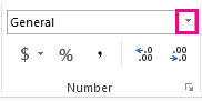
Apply a number format
To distinguish between different types of numbers, add a format, like currency, percentages, or dates.
- Select the cells that have numbers you want to format.
- Click the Home tab, and then click the arrow in the General box.
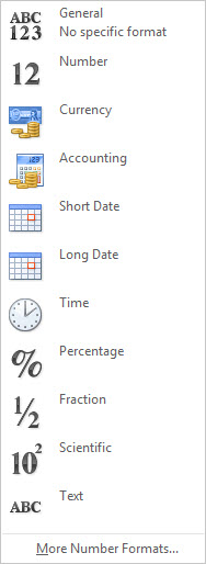
- Pick a number format.
- If you don’t see the number format you’re looking for, click More Number Formats.
Put your data in a table
A simple way to access Excel’s power is to put your data in a table. That lets you quickly filter or sort your data.
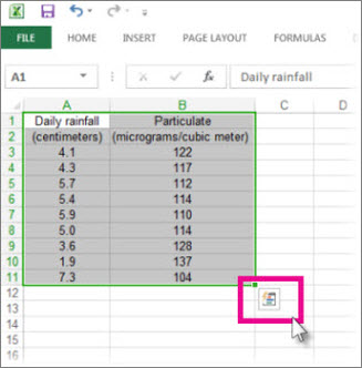
- Select your data by clicking the first cell and dragging to the last cell in your data.To use the keyboard, hold down Shift while you press the arrow keys to select your data.
- Click the Quick Analysis button
in the bottom-right corner of the selection.
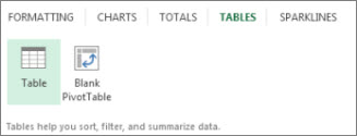
- Click Tables, move your cursor to the Table button to preview your data, and then click the Table button.
- Click the arrow
in the table header of a column.
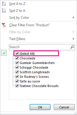
- To filter the data, clear the Select All check box, and then select the data you want to show in your table.
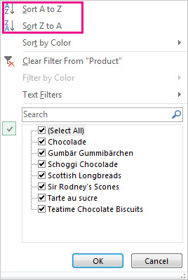
- To sort the data, click Sort A to Z or Sort Z to A.
- Click OK.
Analyse your data
Show totals for your numbers using Quick Analysis
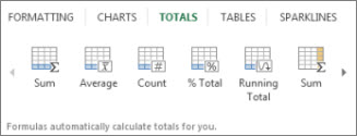
The Quick Analysis tool (Excel 2016) let you total your numbers quickly. Whether it’s a sum, average, or count you want, Excel shows the calculation results right below or next to your numbers.
- Select the cells that contain numbers you want to add or count.
- Click the Quick Analysis button
- Click Totals, move your cursor across the buttons to see the calculation results for your data, and then click the button to apply the totals.
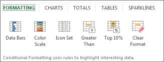
Add meaning to your data using Quick Analysis
Conditional formatting or sparklines can highlight your most important data or show data trends. Use the Quick Analysis tool (Excel 2016) for a Live Preview to try it out.
- Select the data you want to examine more closely.
- Click the Quick Analysis button
in the bottom-right corner of the selection.
- Explore the options on the Formatting and Sparklines tabs to see how they affect your data.
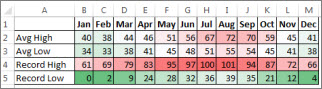
For example, pick a color scale in the Formatting gallery to differentiate high, medium, and low temperatures. - When you like what you see, click that option.
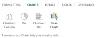
Show your data in a chart using Quick Analysis
The Quick Analysis tool (Excel 2016) recommends the right chart for your data and gives you a visual presentation in just a few clicks.
Click the Charts tab, move across the recommended charts to see which one looks best for your data, and then click the one that you want.
Note: Excel shows different charts in this gallery, depending on what’s recommended for your data.
Select the cells that contain the data you want to show in a chart.
Click the Quick Analysis button in the bottom-right corner of the selection.
Charts and Graphs
Excel Charts and Graphs can be really useful to visualise data and give a clearer picture of what the data can tell you.
Looking at numerous Columns and Rows full of various information can be a bit hard on your eyes and in some cases it just looks meaningless. This is where Charts and Graphs can help by showing the data in a different way, which may result in you spotting some sort of trend or pattern.
To create a Chart or Graph in Excel you’ll first need some data. Following on from the examples above, we have some data relating to restaurant customer numbers and booking numbers for certain dates.
Excel is smart, so if you highlight cells which contain things like a series of dates, headings and data you can go to the ‘Insert’ section, which is located towards the top-left of your screen, and select ‘Recommended Charts’. This will then present you with some appropriate charts and graphs, like so:
Formulas
Excel Formulas can be used to either calculate the value of a single Cell or multiple Cells, as well as use Functions to calculate values or retrieve data.
In Excel, you can use formulas to do basic maths like adding, subtracting, multiplying, and dividing numbers from different cells. You start the formula by entering the equals = symbol. Each type of calculation has its own symbol:
- Use + to add
- Use – to subtract
- Use * to multiply
- Use / to divide
For example, if you wanted to add together the values of three Cells to work out the total value, you could do this:
=B2+C2+D2
To build a formula that adds numbers from different cells, start by selecting the first cell and typing the + symbol. Then, select the second cell and type + again, and finally select the third cell. This creates a formula that adds all three cells together and gives you the total.
This method works well if you’re only adding a few cells. But if you’re working with a lot more, it’s much easier to use the SUM function. This lets you highlight the group of cells you want to add, and Excel will do the rest.
=SUM(B2:D2)
Using the SUM function can save you a lot of time when you’re working with lots of numbers. As you saw in the example above, it works when you highlight many cells in a row — and it also works for cells in a column.
If you need to pull information from different places in your spreadsheet, you can use other functions like VLOOKUP, SUMIF, or COUNTIF. These are helpful when you want to find specific details or get a bigger picture of what your data is showing.
VLOOKUP
Sometimes you’ll need to pull information from one part of your spreadsheet into another — and that’s where functions like VLOOKUP can help.
For example, imagine you’re helping organise a school camp. You’ve got a list of students that includes their names, parent contact details, and which activities they signed up for. Later on, one of your classmates collects everyone’s medical info in a separate list — including any allergies.
Instead of copying and pasting one by one, you can use VLOOKUP to quickly match each student with their allergy information and add it to your original list.
=VLOOKUP(A2,Times!A:B,2,FALSE)
To use VLOOKUP, you need to have something that appears in both of your lists — something Excel can use to match the right rows together. This is called a common identifier, and it must be exactly the same in each list. In our example, the common identifier is the student’s name or email address.
The column that holds this common identifier must be on the left side of the data you’re trying to get. That’s how VLOOKUP knows where to start looking.
Here’s how to build your formula:
- Start by typing
=VLOOKUP( - Then click the lookup value — this is the cell that has the thing you want to match. In our case, it’s the first email address in Cell A2. Then type a comma.
Your formula should now look like this:=VLOOKUP(A2,
- Next, go to the worksheet or tab that has the second list (in our example, it’s called ‘Times’).
- Highlight the columns that include both the lookup value (like the email address) and the data you want (like the arrival time). Then type another comma.
Now your formula looks like this:=VLOOKUP(A2,Times!A:B,
- Then you need to type the column number where the information you want is. This means counting from the first column in the range you just selected. If the arrival time is in the second column, you type 2, then another comma.
Now the formula looks like this:=VLOOKUP(A2,Times!A:B,2,
- Finally, type FALSE. This tells Excel to only find an exact match (which is what you usually want). Then press Enter.
Your final formula should look like this:=VLOOKUP(A2,Times!A:B,2,FALSE)
Once that’s done, you can copy the formula to the rest of the list. Click the small square in the bottom corner of the cell (this is called the Fill Handle) and drag it down. Excel will automatically update the formula for each row and match the correct information.
This is just one way to use VLOOKUP — and it doesn’t have to be with email addresses! You could match students using usernames, ID numbers, or anything that appears in both lists.
SUMIF
Sometimes, you’ll want to add up numbers from a column or row — but only if they meet a certain rule or condition. That’s where the SUMIF function comes in.
For example, imagine you’re helping plan a school fundraising event. You’ve made a list of students who signed up to run different stalls. The list includes their names, the type of stall they chose, and how much money they raised.
Now, if you want to find out how much money was raised just from the food stalls, you can use SUMIF to add up only the amounts that match that category.
=SUMIF(Bookings!D:D,Totals!A2,Bookings!C:C)
Let’s take a closer look at what a SUMIF does. Imagine you’re trying to add up how much money was raised from certain stalls at your school fundraising event — for example, only the food stalls. SUMIF helps you do exactly that.
- First, click the cell under the heading ‘Total Raised’ and type
=SUMIF(. - Then go to the worksheet (in this example, it’s called ‘Fundraising’) that holds your full list of stall data.
- Now select the range — this is the column that has the stall type, because we want to match a specific type like “Food Stall”. After selecting the range, type a comma.
Your formula should now look like:=SUMIF(Fundraising!B:B,
- Next, select the criteria — this is what you’re looking for. In this case, it might be Cell A2, where you’ve written “Food Stall”. Then type another comma.
Now it looks like:=SUMIF(Fundraising!B:B,A2,
- Finally, go back to the ‘Fundraising’ worksheet and select the sum range — this is the column that has the amount of money raised for each stall. Once you’ve selected that, press Enter.
Your full formula should now look like:=SUMIF(Fundraising!B:B,A2,Fundraising!C:C)
Once you’ve done this, you can use the Fill Handle (the little square at the bottom-right of the cell) to drag the formula down. Excel will automatically adjust it for each row, adding up totals based on each type of stall.
This is a quick and easy way to sort and total your data based on specific conditions.
COUNTIF
Sometimes you’ll want to count how many times something appears in your data — like how many times a certain word, number, or date shows up. That’s when you can use the COUNTIF function.
For example, imagine you’ve made a list of students who signed up to help at your school fundraiser. Each row includes their name, the type of stall they’re working on, and the date they’ve signed up for.
If you want to find out how many students signed up for a certain day, you can use COUNTIF to count all the rows that match that date.
=COUNTIF(Bookings!D:D,Totals!A2)